B.A. BA | toby.re

Understanding the radio encoding

We are given a challenge.iq file.

This file is a succession of i and q values as described on wikipedia.

They are a succession of floats encoded on four bytes. We can read them with such a simple python script.

import struct
with open('challenge.iq', 'rb') as f:
    data = f.read()

all_iq = []

print(data[:10])
for k in range(len(data)//8):
    all_iq.append((data[8*k:8*k+4], data[8*k+4:8*k+8]))

print(all_iq[:10])

for iq in all_iq[:10]:
    for k in iq:
        print(struct.unpack('<f', k))

Numpy does it even more easily but at least here we really see what is happening. The numpy equivalent is

npdata = np.fromfile('challenge.iq', dtype=np.float32)

The first thing is to understand how the data is encoded, many different ways of encoding data exist in radio such as

The easiest method to distinguish between all these methods is to trace the (i,q) on a graph and look at the shape.

QAM should show spots on a grid
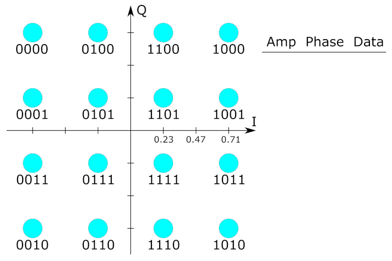
PSK should show a ring of dots
OOK should show two circles, one centered on zero and one higher up

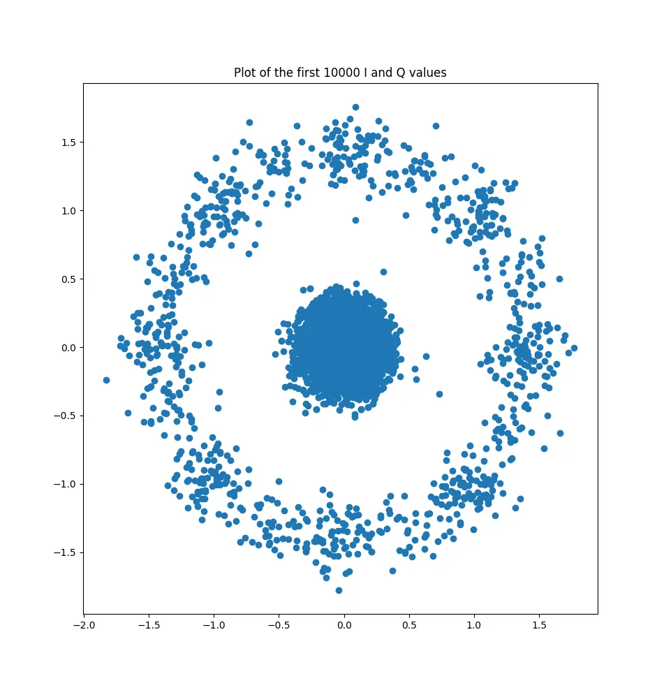
Here we are in the case of OOK. Here is the “constellation graph” of the signal (for the first 10000 values)

And the histogram of the amplitudes histogram of amplitudes

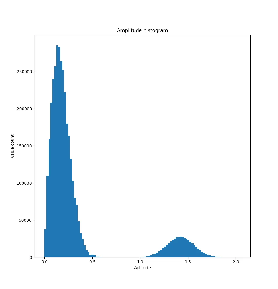
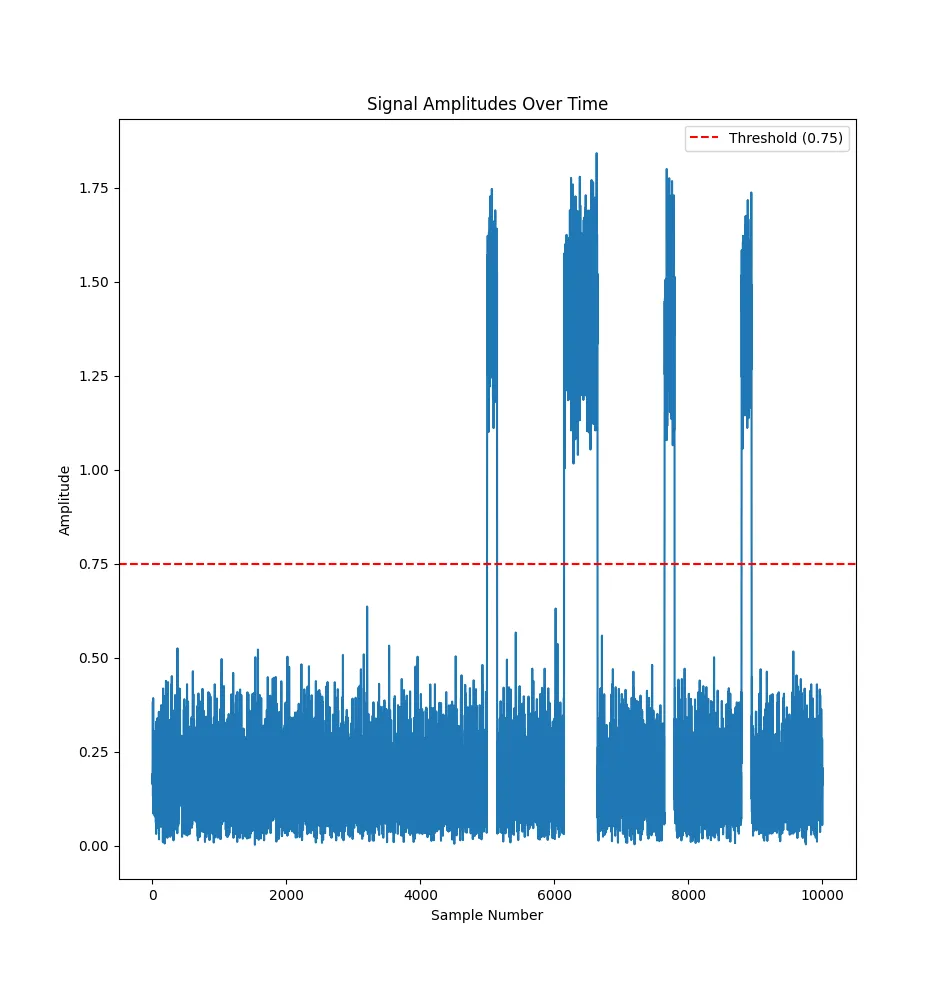
The maximal value seems centered on $\sqrt 2 \approx 1.4$. Let’s plot the beginning of the amplitude variations with a threshold at 0.75. amplitudes over time

Understanding the data encoding

This seems quite clean, so we can write a program to separate the points over and under this threhold, and convert this to binary.

i = npdata[::2]
q = npdata[1::2]
complex_sig = i + 1j * q
magnitudes = np.abs(complex_sig)
binary_data = (magnitudes > 0.77).astype(int)

Now what interest us is the duration of the transitions, to know what is a transmitted 0 and what is a transmitted 1.

Let’s plot the histogram of the durations of each high and low values.

transitions = np.where(np.diff(binary_data) != 0)[0]
plt.hist(np.diff(transitions), bins=200)

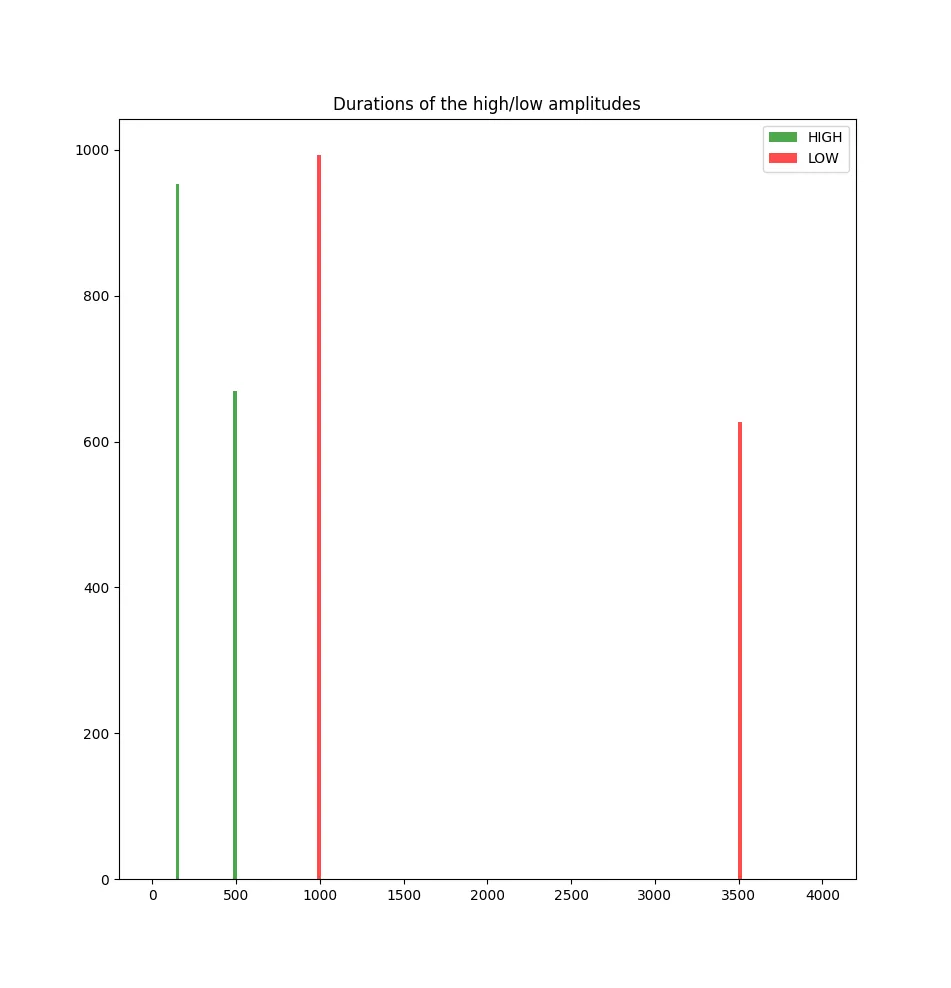
We get this repartition of values histogram of transitions durations

As we can see there are four peaks at a sample rate of 150/500/1000/3500 values. We can guess that :

150 high is 0
500 high is 1
1000 low is a separator between 0 and 1
3500 is a separator between “words”

When we decode this we get these first words:

This looks very much like morse code with a 0 being a dot and a 1 a dash (the first letters being understandalbe as LE CODE MORS)

We can decode this into

import numpy as np

iq = np.fromfile('challenge.iq', dtype=np.float32)
states = np.abs(iq[::2] + 1j * iq[1::2]) > 0.77

changes = np.where(np.diff(states))[0]
durations = np.diff(np.insert(changes, 0, 0))

output = ''
for is_on, d in zip(states[changes], durations):
    if is_on:
        if 100 < d < 250: output += '0'
        elif 400 < d < 600: output += '1'
    else:
        if d > 2000: output += '\n'
        elif d > 800: output += ' '

morse = {
    '01': 'A', '1000': 'B', '1010': 'C', '100': 'D', '0': 'E',
    '0010': 'F', '110': 'G', '0000': 'H', '00': 'I', '0111': 'J',
    '101': 'K', '0100': 'L', '11': 'M', '10': 'N', '111': 'O',
    '0110': 'P', '1101': 'Q', '010': 'R', '000': 'S', '1': 'T',
    '001': 'U', '0001': 'V', '011': 'W', '1001': 'X', '1011': 'Y',
    '1100': 'Z', '01111': '1', '00111': '2', '00011': '3', '00001': '4',
    '00000': '5', '10000': '6', '11000': '7', '11100': '8', '11110': '9',
    '11111': '0',
}

decoded = ''
for line in output.strip().split('\n'):
    k = line.replace(' ', '')
    decoded += morse.get(k, ' ' if not k else '?')

print(decoded)
""" LECODEMORSEINTERNATIONALOULALPHABETMORSEINTERNATIONALESTUNCODEPERMETTANTDETRANSMETTREUNTEXTEALAIDEDESERIESDIMPULSIONSCOURTESETLONGUESQUELLESSOIENTPRODUITESPARDESSIGNESUNELUMIEREUNSONOUUNGESTESTOPCECODEESTSOUVENTATTRIBUEASAMUELMORSECEPENDANTPLUSIEURSCONTESTENTCETTEPRIMAUTEETTENDENTAATTRIBUERLAPATERNITEDULANGAGEASONASSISTANTALFREDVAILSTOPLEFLAGESTE6891C8BB8CCFE95A767457F3A1B73861928A002C5094762D580CD7BC4A15C64STOPINVENTEEN1832POURLATELEGRAPHIECECODAGEDECARACTERESASSIGNEACHAQUELETTRECHIFFREETSIGNEDEPONCTUATIONUNECOMBINAISONUNIQUEDESIGNAUXINTERMITTENTSSTOPLECODEMORSEESTCONSIDERECOMMELEPRECURSEURDESCOMMUNICATIONSNUMERIQUESSTOP
"""

Now the flag must be put in lowercase so

echo "FCSC{$(echo 'E6891C8BB8CCFE95A767457F3A1B73861928A002C5094762D580CD7BC4A15C64' | tr '[:upper:]' '[:lower:]')}"

Plotting scripts

These are the scripts I used to plot the values

import matplotlib.pyplot as plt
import numpy as np

# import struct
# with open('challenge.iq', 'rb') as f:
#     data = f.read()
#
# all_iq = []
#
# print(data[:10])
# for k in range(len(data)//8):
#     all_iq.append((data[8*k:8*k+4], data[8*k+4:8*k+8]))
#
# print(all_iq[:10])
#
# for iq in all_iq[:10]:
#     for k in iq:
#         print(struct.unpack('<f', k))

npdata = np.fromfile('challenge.iq', dtype=np.float32)

i = npdata[::2]
q = npdata[1::2]

num_samples = 10000
plt.scatter(i[:num_samples], q[:num_samples])
plt.title(f'Plot of the first {num_samples} I and Q values')
plt.show()

complex_sig = i + 1j * q

magnitudes = np.abs(complex_sig)

plt.hist(magnitudes, bins=100)
plt.title('Amplitude histogram')
plt.xlabel('Aplitude')
plt.ylabel('Value count')
plt.show()

magnitudes_slice = magnitudes[:num_samples]

plt.plot(magnitudes_slice)

threshold = 0.75
plt.axhline(y=threshold, color='red', linestyle='--', label=f'Threshold ({threshold})')

plt.title('Signal Amplitudes Over Time')
plt.xlabel('Sample Number')
plt.ylabel('Amplitude')
plt.legend()
plt.show()

binary_data = (magnitudes > 0.77).astype(int)

transitions = np.where(np.diff(binary_data) != 0)[0]

plt.hist(np.diff(transitions), bins=200)
plt.title('0/1 durations')
plt.show()

And for the transitions durations:

import numpy as np
import matplotlib.pyplot as plt

iq = np.fromfile('challenge.iq', dtype=np.float32)
states = np.abs(iq[::2] + 1j * iq[1::2]) > 0.77

changes = np.where(np.diff(states))[0]
durations = np.diff(np.insert(changes, 0, 0))
values = states[changes]

high_durations = durations[values]
low_durations = durations[~values]

bins = np.linspace(0, 4000, 200)

plt.hist(high_durations, bins=bins, color='green', alpha=0.7, label='HIGH')
plt.hist(low_durations, bins=bins, color='red', alpha=0.7, label='LOW')
plt.legend()
plt.title('Durations of the high/low amplitudes')
plt.show()